
In my Digital Image Processing course, we were tasked with a challenging project. The goal was to create a system capable of analyzing images of six different plant species. The system had to be trained using a dataset of 36 images, and once trained, it should be able to analyze all images in a specified folder. The final output of the system was to generate a comprehensive report containing information about each analyzed image, including the name of the image file. In the following sections, I will detail how I approached and solved this problem.
Getting to Know Our Leafy Subjects: An Introduction to the Dataset
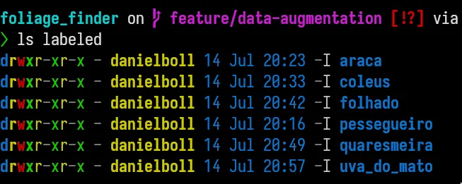
The first thing we needed to do in this project was getting to grips with the dataset. We had 36 images, each packed with different plant species – six in total. However, there was a hitch. None of the images were labeled. So, all we had were a bunch of leaf images from various plants, without any indications of which leaf belonged to which plant.
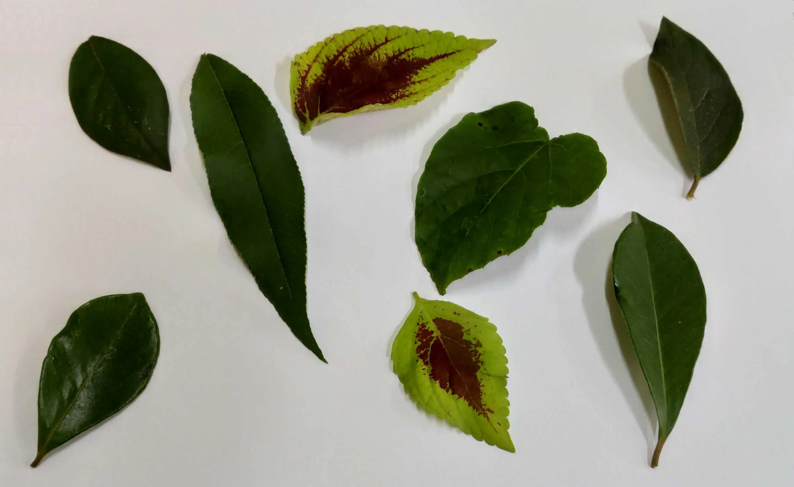
Figure 1: A image from the dataset
Here’s an example image from the dataset. As you can see, it’s not immediately clear which leaf belongs to which plant species. We were truly in uncharted territory.
The Problem: Tackling an Unlabeled Dataset and Close Neighbors
Working with an unlabeled dataset was our first hurdle. Most of my prior machine learning experience had been with supervised learning, where you have clear labels for training data. But in this case, we had to get our hands dirty and dive into the deep end of unsupervised machine learning.
Our task was to label the data manually, which meant separating each leaf from the images and then assigning them a label. And if that wasn’t enough, some leaves were too close together, which made them hard to separate. Picture two pieces of paper glued together, and you get the idea.
Creating the Environment: Welcome to the Python World
The next step in our journey was to set up our working environment. We decided to use Python, a favorite in the machine learning realm, for its simplicity and robustness. Plus, it’s got a treasure trove of useful libraries and tools, making it an excellent choice for this project.
To create a consistent and portable development environment, we used Docker. This allowed us to package up the application with all of the parts it needed and run it anywhere Docker is installed. Below is the Dockerfile we used:
# Use an official Tensorflow runtime as a parent image
FROM tensorflow/tensorflow:latest-gpu-jupyter

# Set the working directory to /app
WORKDIR /app

# Add local directory's content to the docker image under /app
ADD . /app

# Allow statements and log messages to immediately appear in the Knative logs
ENV PYTHONUNBUFFERED True

RUN apt-get update && apt-get install -y \
    wget \
    libcairo2-dev \
    libgl1-mesa-glx \
    python3-tk

# Install any needed packages specified in the requirements file
COPY requirements.txt /app
RUN pip install --no-cache-dir -r requirements.txt
We used the official Tensorflow image as our base and installed some additional packages that we needed. We also copied our local directory content into the docker image and installed the necessary Python packages from our requirements.txt file.
At the start, our project was without a requirements.txt, the lifeline of Python dependencies. An attempt to create one with pip freeze fell flat (image analysis can be picky!). So, we found ourselves manually jotting down dependencies as we progressed. Ah, the joy of unexpected surprises in coding! Should have used Poetry.
To manage our Docker environment more easily, we used Docker Compose. Here’s the docker-compose.yml file we used:
version: "3"

services:
  tensorflow:
    build: .
    volumes:
      - .:/app
    ports:
      - "5000:5000"
    command: /bin/bash
With this setup, we were able to persist our data across Docker sessions, as Docker Compose takes care of the volumes for us.
Finally, we created a Makefile to automate our common tasks, such as building the Docker image, running the Docker container, and running our main Python script:
.PHONY: build run sudo_run help

help: ## Show this help
 @echo "Available targets:"
 @echo
 @awk 'BEGIN {FS = ":.*?## "} /^[a-zA-Z_-]+:.*?## / {printf "\033[36m%-15s\033[0m %s\n", $$1, $$2}' $(MAKEFILE_LIST)

build: ## Build the Docker image
 docker-compose build

run: ## Run the Docker container
 docker-compose run -u $(shell id -u):$(shell id -g) tensorflow bash

sudo_run: ## Run the Docker container as sudo
 docker-compose run tensorflow bash

drun: clean ## Run the code within the docker
python src/main.pySweet AWK juice to make a automatic help message in Make.
Pruning the Dataset: Separating the Leaves
After setting up our environment and sorting out our dependencies, it was time to roll up our sleeves and start the real work. The first major task? Implementing the leaf extraction.
The goal here was to segment the leaves in the images, isolate them from each other, and then save them separately for further analysis. This process is crucial, as it ensures our machine learning model can focus on individual leaves, rather than being confused by a bunch of overlapping leaves.
import os
import cv2
import numpy as np

def extract_leaves(image_path, output_folder):
    os.makedirs(output_folder, exist_ok=True)
    min_area_threshold = 100
Our function extract_leaves{:python} takes two arguments: the path to the image file and the output folder to save extracted leaves. The os.makedirs(output_folder, exist_ok=True){:python} line ensures the output folder is created if it doesn’t exist. We also set a minimum area threshold to ignore any small areas that could be noise.
def extract_leaves(image_path, output_folder):
    os.makedirs(output_folder, exist_ok=True)
    min_area_threshold = 100

    img = cv2.imread(image_path, cv2.IMREAD_UNCHANGED)
    channels = cv2.split(img)
We load the image using cv2.imread{:python} with the flag cv2.IMREAD_UNCHANGED{:python} to preserve transparency information. Then, we split the image into its channels (Red, Green, Blue, Alpha) using cv2.split{:python}.
def extract_leaves(image_path, output_folder):
    os.makedirs(output_folder, exist_ok=True)
    min_area_threshold = 100

    img = cv2.imread(image_path, cv2.IMREAD_UNCHANGED)
    channels = cv2.split(img)

    _, mask = cv2.threshold(channels[3], 1, 255, cv2.THRESH_BINARY)
We create a mask by thresholding the alpha channel (the 4th channel in our image). The cv2.threshold function sets all pixel values greater than 1 to 255 (white), creating a binary image where the leaves are white and the background is black.
def extract_leaves(image_path, output_folder):
    os.makedirs(output_folder, exist_ok=True)
    min_area_threshold = 100

    img = cv2.imread(image_path, cv2.IMREAD_UNCHANGED)
    channels = cv2.split(img)

    _, mask = cv2.threshold(channels[3], 1, 255, cv2.THRESH_BINARY)

    contours, _ = cv2.findContours(mask, cv2.RETR_EXTERNAL, cv2.CHAIN_APPROX_SIMPLE)
Then, we find the contours (outlines) of all objects in the mask using the cv2.findContours function. This gives us a list of contours, each representing a leaf in the image.
    img = cv2.imread(image_path, cv2.IMREAD_UNCHANGED)
    channels = cv2.split(img)

    _, mask = cv2.threshold(channels[3], 1, 255, cv2.THRESH_BINARY)

    contours, _ = cv2.findContours(mask, cv2.RETR_EXTERNAL, cv2.CHAIN_APPROX_SIMPLE)

    for i, contour in enumerate(contours):
        area = cv2.contourArea(contour)
        if area < min_area_threshold:
            continue
We loop through each contour and calculate its area using cv2.contourArea. If the area is smaller than our set threshold, we skip the contour. This helps us ignore small noises or artifacts in the image.
    for i, contour in enumerate(contours):
        area = cv2.contourArea(contour)
        if area < min_area_threshold:
            continue

        contour_mask = np.zeros_like(mask)
        cv2.drawContours(contour_mask, [contour], 0, 255, -1)
        object_img = cv2.bitwise_and(img, img, mask=contour_mask)
For each valid contour, we create a blank mask and draw the contour on it using cv2.drawContours. This gives us a mask where only the current leaf is white. We then perform a bitwise-and operation on the original image and the mask, effectively isolating the leaf in the image.
    for i, contour in enumerate(contours):
        area = cv2.contourArea(contour)
        if area < min_area_threshold:
            continue

        contour_mask = np.zeros_like(mask)
        cv2.drawContours(contour_mask, [contour], 0, 255, -1)
        object_img = cv2.bitwise_and(img, img, mask=contour_mask)

        image_file = os.path.basename(image_path)
        object_name = f"{os.path.splitext(image_file)[0]}_{i}.png"
        output_path = os.path.join(output_folder, object_name)
        cv2.imwrite(output_path, object_img)
Finally, we save each isolated leaf as a separate image in our output folder. We generate the output file name based on the original image’s name and the index of the contour, ensuring each leaf gets a unique name.
This function was key to preparing our dataset for further processing.
| Pre-pruned images | Pruned images |
|---|---|
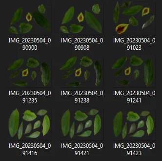 | 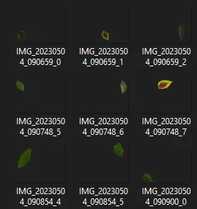 |
Good Ol’ Manual Labeling: A Sip of Coffee and a LOT of Patience
Once we extracted the individual leaves from each image, we had another challenge to tackle - labeling. You’d think we had some complex, fancy-pants algorithm do the job, right? Well, not really!
We simply labeled each leaf by eye and hand, old-school style. Yep, that’s right! It’s like playing ‘spot the differences’, only with leaves and, trust me, they aren’t as different as you’d hope. Every leaf took a sip of coffee and a squinty-eyed look, backed up by some educated guesses (and prayers).
A little bit of drudgery? Absolutely. But hey, nothing says ‘hands-on data science’ quite like manually labelling hundreds of leaf images while nursing a caffeine overdose. So, a toast to the unsung hero of any machine learning project - the humble manual labeler! (The things we do for love… and accuracy).
Remember folks, machine learning isn’t all glamorous algorithms and fancy models. Sometimes, it’s about slogging through leaf pictures while questioning your life choices.
Feature Extraction: The ‘What’s What’ of Leaves
With our leaves neatly isolated, we moved on to the critical step of feature extraction. Here’s a look at the code that performed this task:
def extract_feature(image_path, step=Step.TRAIN):
    features = {}

    # Get the original contours and extract features
    contours = image.get_contours(image_path)
    features[image_path] = extract_features_from_contours(
        contours, image_path, step)

    return features
In our extract_feature{:python} function, we find the leaf contours and then extract the features from these contours. The extracted features are stored in a dictionary using the image path as the key.
def extract_features_from_contours(contours, image_path, step):
    contour_features = []

    freeman_features = freeman_chain_code.extract_features(contours)
    statistical_features = statistics.extract_features(contours)
    local_binary_pattern_features = local_binary_pattern.extract_features(
        contours, image_path)

    for freeman_feature, statistical_feature in zip(freeman_features,
                                                    statistical_features):
        feature = {
            "chain_code": freeman_feature,
            "lbp": local_binary_pattern_features,
            **statistical_feature,
        }

        if step == Step.TRAIN:
            name = image_path.split("/")[1]
            feature["class"] = name

        contour_features.append(feature)

return contour_featuresAs we can see only when we are training the model we do know the classes.
Feature Serialization: Storing the Leafy Knowledge
Once we have successfully extracted the critical features from our leaf dataset, the next step is to serialize and store this data. Serializing our dataset converts it into a format that can be easily saved to disk and subsequently loaded back when needed. For this purpose, we use a powerful Python library known as joblib.
Here’s a simple piece of code demonstrating how we’ve done this:
from joblib import dump, load

def save_features(features):
    dump(features, "features.pkl")

def load_features():
    return load("features.pkl")
And just like that, our feature extraction process is complete! We’ve successfully isolated our leaves, extracted meaningful features from them, and stored these features for future use.
Model Training: Teaching our AI to Understand Leaves
So, you’ve followed us through leaf isolation and feature extraction, and we’ve managed to store all this data in a convenient format. But what next? Here comes the exciting part – training our model! In this section, we’ll get our hands dirty with some real machine learning using a type of network known as a Multi-Layer Perceptron (MLP).
Let’s walk through the code that does the magic:
import numpy as np

from sklearn.model_selection import train_test_split
from sklearn.neural_network import MLPClassifier
from sklearn.preprocessing import StandardScaler

def train(features):
    X = []
    y = []

    # Extract the features and their respective classes
    for _, v in features.items():
        for d in v:
            for i in range(len(d["extent"])):
                feature = [
                    d["aspect_ratio"][i],
                    d["eccentricity"][i],
                    d["extent"][i],
                    d["solidity"][i],
                    *d["hu_moments"][i],
                    *d["lbp"][i],
                ]

                X.append(feature)
                y.append(d["class"])

    # Convert the lists to numpy arrays
    X = np.array(X)
    y = np.array(y)

    # Scale your data
    scaler = StandardScaler()
    X = scaler.fit_transform(X)

    # Split into train and test sets
    X_train, X_test, y_train, y_test = train_test_split(
        X,
        y,
        test_size=0.3,
        random_state=42,
        stratify=y,
    )

    # Create the MLP classifier
    mlp = MLPClassifier(hidden_layer_sizes=(100, 100),
                        max_iter=200,
                        verbose=True)

    # Fit the model
    mlp.fit(X_train, y_train)

    # Save the model
    dump(mlp, "model.pkl")
Now, I understand that it might not be the prettiest code you’ve ever seen. But hey “if it looks stupid but it works, it ain’t stupid!”.
This function, aptly named train, takes in our pre-processed features as input. It prepares the data, scales it, splits it into training and testing sets, and then trains our MLP model. Finally, the trained model is saved to the disk for future use.
The model training process involves a few steps:
- We first construct our feature matrix X and target vector y.
- The feature data is then standardized to ensure that our MLP isn’t swayed unduly by features that naturally have larger values.
- Our data is split into a training set to teach our model and a test set to verify its performance. We’re reserving 30% of the data for testing purposes.
- An MLPClassifier object is then initialized with two hidden layers, each having 100 neurons. The training process is carried out over 200 iterations (epochs).
- The model is then trained using the fit method, and we finally save our trained model to a file named model.pkl for future use.
The beauty of coding isn’t just about creating intricate and aesthetically pleasing lines of code. It’s about getting the job done, and our humble piece of training code does just that – efficiently, and effectively!
Classification: Bringing the AI to Life with Labels
The model training chapter has been a roller coaster, and now we have a trained model ready to unleash on leaf images. The next exciting chapter is about the classification, where our trained Multi-Layer Perceptron (MLP) takes in the processed features and recognizes the types of leaves.
Here’s how the magic unfolds:
Loading the Trained Model
First, we load our previously saved MLP model from the disk.
mlp = load("model.pkl")Preparing the Features
We loop through the files, extract the features, and construct our feature matrix X just like we did in the training process.
for file in files:
    X = []
    for d in features[file]:
        lbp_feature = list(chain(*d["lbp"]))
        feature = [
            d["aspect_ratio"],
            d["eccentricity"],
            d["extent"],
            d["solidity"],
            *d["hu_moments"],
            *lbp_feature,
        ]
        X.append(feature)

    # Convert the lists to numpy arrays
    X = np.array(X)
Scaling and Prediction
The features are then standardized, and the MLP model predicts the classes along with the probabilities for each class.
# Scale your data
scaler = StandardScaler()
X = scaler.fit_transform(X)

# Predict the classes
predictions = mlp.predict(X)
probabilities = mlp.predict_proba(X)
Labeling the Images
The predictions and probabilities are then used to annotate the original images with labels. The bounding rectangles and labels are drawn on the images.
image = cv2.imread(file)
probability_of_class = np.max(probabilities, axis=1)
for i, leaf_features in enumerate(features[file]):
# Get the bounding rectangle and calculate the label positions
# Draw the text labels and percentage labels on the image
print(f"Label: {predictions[i]} with probability {probability_of_class[i]}")
print("Features:")
leaf_contour = leaf_features["contours"][i]
# Get the bounding rectangle
x, y, w, h = cv2.boundingRect(leaf_contour)
# Calculate the center of the rectangle
class_label = (x + w // 2, y + h // 2)
percentage_label = (x + w // 2, y + h // 2 + 40)
# Draw the text label on the image
cv2.putText(
image,
str(predictions[i]),
class_label,
cv2.FONT_HERSHEY_SIMPLEX,
1,
(0, 255, 0),
2,
)
# Draw the percentage label on the image
cv2.putText(
image,
f"{probability_of_class[i] * 100:.2f}%",
percentage_label,
cv2.FONT_HERSHEY_SIMPLEX,
1,
(255, 255, 0),
2,
)
# Save the classified image
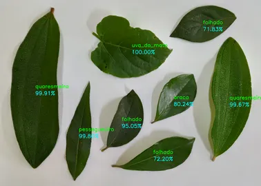
cv2.imwrite("classified/" + file.split("/")[-1], image)The result is an image where each leaf is labeled with its corresponding class and confidence score.
The classification step is where the AI showcases its intelligence, turning raw data into insights. It is the final piece that completes the puzzle, letting us see the leaves through the lens of our intelligent algorithm.
This brings us to the end of our AI journey to understand leaves. We’ve learned about preprocessing, feature extraction, model training, and classification. Now you have a full-fledged system capable of recognizing and labeling different types of leaves. Happy leaf hunting! 🍁